Exploring Gradient Descent and Its Variants

This article is written based on the lecture MATH532 by Prof. Hwang at POSTECH.

What is Gradient Descent Algorithm

In machine learning, we usually have to find a way to minimize a traget function (e.g. MSE). How can we find the minimum of the target function if it is too dizzy to find the minimum? Think about the basic calculus which you learned in your freshman. There was a notion called “Gradient,” which points the dirction of the steepest slope. Its magnitude also means the rate of increase or decrease of the function in the direction. Therefore, gradient is very of use to find minimum or maximum valu in that it points where we have to go to find our destination. Of course, we have to follow the direction where gradient points. This can be written as

$$w_k = w_{k-1} - \eta \cdot \nabla_w J(w_{k-1}) = w_{k-1} - \eta \cdot \nabla_w \sum_{i=1}^{N} L(w_{k-1};x_i,y_i)$$

where $J(w) = \sum_{i=1}^{N}L(y_i,\hat{f}(w;x_i))$ and $L$ is a loss function.

Limitations

Simple gradient descent alogrithm has several limitations.

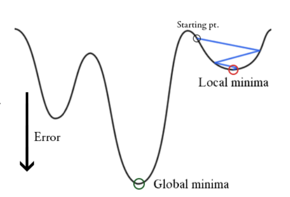
• If the starting point for gradient descent was chosen inappropriately, the algorithm will only make it approach a local minimum, never reaching the global one.

• We need to compute $\nabla_w L(w_{k-1};x_i,y_i)$for all $i$ to perform one update. Hence, it can be very slow and is intractable for datasets that don’t fit in memory.

Stochastic Gradient

One method to overcome the limitations alluded before is the stochastic gradient descent. It is literally the stochastic approximation of gradient descent optimization.

We select data size $B$ from all sample size $N$. Then we can iteratively calculate parameter $w$ where the loss function is being minimized. This can reduce the computational burden. Also, there is a fluctuation in the objective function since we select the $B$ data randomly. This fluctuation enables it to jump to new and potentially better local minima.

$$w_k = w_{k-1} - \eta \cdot \nabla_w \sum_{i=1}^{B} L(w_{k-1};x_i,y_i)$$

Momentum Methods

This is the most interesting algoritm in the class today! When we drop the ball on the complex loss function with a proper friction, the ball is likely to pass through the local minima and arrive at global minima. This is becuase as ball moves downward, its potential energy transform to the kinetic energy so that it gains the energy to pass through the local minima. Momentum Methods are made inspired by this physical phenomenon. The name momentum comes from the fact that the negative gradient is a force moving a particle through parameter space. (although it is not exactly the same as that found in classical momentum.)

The algorithm can be expressed with equations as below.

$$v_k = \gamma v_{k-1} + \eta \cdot \nabla_w \sum_{i=1}^{B} L(w_{k-1};x_i,y_i)$$ $$w_k = w_{k-1} - v_k \newline= w_{k-1} - \eta \cdot \nabla_w \sum_{i=1}^{B} L(w_{k-1};x_i,y_i)$$

Here, $\gamma$ plays a role as a friction. (Although not exactly same.) It is a method that helps acclerate SGD (Sotchasstic Gradient Descent) in the relevant direction and dempens oscillations. Also, it can hlep to escape local minima.

Nestrov Accelerated gradient

Momentum method adjusts the momentum based on current position $w_{k-1}$. On the other hand, Nestrov Acclerated gradient based on approximated future position $w_{k-1}-\gamma w_{k-1}$.

$$v_k = \gamma v_{k-1} + \eta \cdot \nabla_w \sum_{i=1}^{B} L(w_{k-1}-\gamma w_{k-1};x_i,y_i)$$ $$w_k = w_{k-1} - v_k \newline= w_{k-1} - \eta \cdot \nabla_w \sum_{i=1}^{B} L(w_{k-1}-\gamma w_{k-1};x_i,y_i)$$

Adaptive Method

AdaGrad

As I alluded before, in order to arive at global minimum, not local minimum, we need to have appropriate parameter $\eta$. Too small $\eta$ can cause too slow convergence and too small $\eta$ can cause too much fluctuation to converge. Also having a constant $\eta$ is not suitable in the complex loss function.

AdaGrad (Adaptive Gradient) is the algorithm that djust learning rate automatically. It updates more for infrequent parameter and less for frequent parameter. The algorithm can be written as $$g_{k-1,i} := \nabla_w J(w_{k-1})$$

$$G_{k-1,i} = \sum_{t=0}^{k-1}|g_{t,i}|^2$$

$$w_k = w_{k-1} - \eta \cdot \nabla_w \frac{\eta}{\sqrt{G_{k-1.i+\epsilon}}}g_{k-1,i}$$

As the accumulated gradient gets bigger, the learning rate gets smaller.

RMSProb

AdaGrad has some weaknesses because denominator $G$. Since $G$ increases monotonically, the learning rate becomes shrink and eventually becomes very small so the algorithm can not learn anymore. If we change the summation of $g_{k-1,i}$ into the average of $g_{k-1,i}$, the problem can be solved. RMSProb average previous $g$ and current $g$ with the weight $1-\gamma$ and $\gamma$ respectively.

$$g_{k-1,i} := \nabla_w J(w_{k-1})$$

$$E[g^2]_{k-1} = \gamma E[g^2] _{k-1} + (1-\gamma) g^2 _{k-1}$$

where $$E[g^2]_{k-1} = \sum^{k-1} _{i=0}(1-\gamma)\gamma^i g^2 _{k-1-i}$$

and $$w_k = w_{k-1} - \eta \cdot \nabla_w \frac{\eta}{\sqrt{E[g^2]_{k-1}+\epsilon}}g_{k-1,i}$$

AdaDelta

AdaDelta is another extension of AdaGrad. AdaDelta not only focuses on the denomiantor but also numerator.

$$g_{k-1,i} := \nabla_{w_k} J(w_{k-1})$$

$$E[\Delta w^2]_{k-1} = \gamma_1 E[\Delta w^2] _{k-2} + (1-\gamma_1) \Delta w^2 _{k-1}$$

$$E[g^2]_{k-1} = \gamma_2 E[g^2] _{k-1} + (1-\gamma_2) g^2 _{k-1}$$

and $$w_k = w_{k-1} - \eta \cdot \nabla_w \frac{\sqrt{E[\Delta w^2]_{k-1}+\epsilon}}{\sqrt{E[g^2]_{k-1}+\epsilon}}g_{k-1,i}$$

Adam

Adam is the algorithm that mixes RMSProp and Momentum. It was proposed by KIngma &Ba. It not only keeps the average of past squared gradients like Adadelta and RMSProp, but also keep the average of past gradients. Since inital average are biased towards zero, Adam adjusts initial averages to be unbiased.

$$g_{k-1,i} := \nabla_{w_k} J(w_{k-1})$$

$$m_{k-1} = \gamma_1 m_{k-2} + (1-\gamma_1)g_{k-1}$$

$$v_{k-1} = \gamma_2 v_{k-2} + (1-\gamma_2)g^2_{l-1}$$

$$\newline \newline \hat{m_{k-1}} = \frac{m_{k-1}}{1-\gamma^{k-1}_1}$$

$$\hat{v_{k-1}} = \frac{v_{k-1}}{1-\gamma^{k-1}_2}$$

and $$w_k = w_{k-1} - \frac{\eta}{\sqrt{\hat{v}_{k-1}}+\eta} \hat{m} _{k-1}$$

Code

You can get the gradient descent code I wrote from scratch.

https://github.com/MunjungKim/Gradient-Descent-Algorithm

Reference

• Hastie, T., Tibshirani, R., & Friedman, J. (2009). The Elements of Statistical Learning: Data Mining, Inference, and Prediction, Second Edition. New York: Springer Series in Statistics

• James, G., Witten, D., Hastie, T., & Tibshirani, R. (2013). An introduction to statistical learning (Vol. 112). New York: springer.